GRID3 COD - Roads v1.0 Data Release Notes

Field	Value
Name of the dataset	GRID3 COD - Roads v1.0
Name of the file	GRID3_COD_roads_v1_0.gpkg
Date of data release	January 08, 2026
File format	OGC Geopackage
Dataset version	v1.0
Abstract	This document outlines the methodology and data sources used to produce the GRID3 COD - Roads v1.0 dataset. The spatial dataset consists of road and path locations in the Democratic Republic of the Congo.
Dataset citation	Center for Integrated Earth System Information (CIESIN), Columbia University. 2026. GRID3 COD - Roads v1.0. New York: Columbia University. https://doi.org/10.7916/00gb-e164. Accessed <DAY MONTH YEAR>.
Terms of use	Users are free to download, store, access, use, copy, adapt, transform, alter, arrange, build upon, distribute and transmit this work and any derivative works. Attribution of the source must be provided, and further distribution of this work or derived work must maintain the same terms of data use and license as set forth in this Terms of Use. Copyright 2026. The Trustees of Columbia University in the City of New York.
Data license	The data and accompanying document are licensed under a Creative Commons Attribution-ShareAlike 4.0 International, CC BY-SA 4.0 (https://creativecommons.org/licenses/by-sa/4.0/) and specified in legal code (https://creativecommons.org/licenses/by-sa/4.0/legalcode).
Contacts and data queries	The authors of this dataset appreciate feedback regarding the data, including suggestions, discovery of errors, difficulties in using the data, and format preferences. For dataset-related questions, please send an email to: info@ciesin.columbia.edu

1 Input datasets

Multiple input data were used to create the GRID3 COD - Roads v1.0, see table 1 below.

1.0.1 Table. Data inputs

Name	Data Type/Format	Release Year	Input Data Year	Source Acronym
Meta (Open Mapping at Facebook)	Road segments	2020	2020	CIESIN / Meta
GPS Track Data	GPS Tracking points	2025	2019-2025	GRID3 / CIESIN
COD GRID3 Settlement Extents v3.1	Settlement polygons	2024	2016 - 2023	n/a
Overture Maps Foundation	Road segments	2025	varies	Overture / OSM
OpenStreetMap Water Bodies, downloaded from Geofabrik on 09/04/2025	Lines and polygons representing water bodies	2025	varies	n/a
Copernicus GLO-30 Digital Elevation Model (DEM) at 30 m resolution¹	raster	2019	2010-2015	n/a
Land use/ land cover (LULC) from ESRI’s Living Atlas, using Sentinel-2 data, at 10 m resolution	raster	2024	2024	n/a

NEED TO ADD LINKS TO TABLE ENTRIES

2 Methodology

2.1 Road Data Integration and Cleaning

The GRID3 COD roads dataset integrates three primary sources: Overture Roads data (derived from OpenStreetMap), road feature extractions from satellite imagery conducted by Meta (formally Facebook) in 2020, and GPS track data collected during field campaigns and GRID3 fieldwork. The Overture data serve as the foundational layer of the dataset and were incorporated in full, without any modifications to the geometries. In cases where Meta or GPS tracks overlapped with Overture, Overture was preferred, and in cases where GPS tracks overlapped with Meta, Meta was preferred. Both Meta and roads derived from GPS tracks were used to fill the gaps, complementing the dataset in areas not covered by Overture.

To incorporate Meta and GPS track data into a usable road network, topological corrections were necessary. Road network models require a specific topology that defines how the line segments (roads) connect to each other and to the nodes (intersections or endpoints). First, Meta roads were merged with Overture roads by snapping to the nearest Overture segments within a 1-meter tolerance. Next, Meta segments were snapped to other Meta segments within a 3-meter tolerance.

GPS track points were used to construct travel paths based on the temporal information and device ID associated with a track (Figure 1). To remove noise created by GPS error, track data was cleaned to drop any consecutive points where travel speed was faster than 100 km/h, ping time was greater than 30 minutes, or the distance travelled was greater than 1,000-m. Track points were then converted to linear track segments. Next, we removed track segments that were close to each other, but disconnected by creating 100-m buffers around segments which were dissolved and converted from multipart to singlepart features. For each buffer feature, we created a centerline. To remove track segments that duplicated existing roads, the resulting centerlines were discarded if they overlapped more than 70% with a 300 m buffer created around Overture/Meta roads. The remaining line features were aligned with both Overture and Meta roads with a tolerance of 250-m. To enable node creation, vertices were added to the Meta road and GPS track segments using the Integrate tool. These segments were then split at the nodes using dissolve and converted back to singlepart features.

We found several cases where Meta’s extractions were misclassified–likely due to interference from clouds or other natural features (Figure 2). Additionally, track roads contained noise due to GPS error. To filter out erroneous road segments, the remaining Meta roads and GPS tracks were further cleaned by creating a settlement-network connecting GRID3 Settlement polygons along Overture, Meta, and track roads (Figure 3). Lines generated to connect settlements along the road network were done so using the Optimal Region Connections tool in ArcGIS Pro and are referred to as optimal paths. Meta roads that were not either within a settlement or useful in connecting a settlement to other roads in the network were removed. GPS tracks were also removed if they were not within a settlement, useful for connecting a settlement, or did not connect two segments of Overture/Meta roads. This settlement-network cleaning was conducted based on the assumption that roads should connect populated areas, thus unconnected, stand-alone segments may be less likely to represent an actual road. Even when removed road segments were valid roads, many were used to get to fields and not for navigation between populated areas.

To create a more connected road network, an additional segment type was derived from optimal paths created in the settlement-network. Optimal segments were kept if they were necessary for connecting the endpoints of two previously unconnected road segments. Optimal segments were aligned with the other roads using a 10-m tolerance. Roads created from optimal paths can be identified through the source_id attribute and are labelled as “CIESIN”. The class assigned to these road segments is derived from the connected Meta, Overture, or GPS track segments. The classes of Overture and Meta were retained from the source data and GPS track classes were set to unknown except for those identified as “water tracks”.

A unique subset of tracks representing travel along water were identified as tracks that overlapped more than 70% with OSM water polygons. While these water tracks do not represent traditional roads, they represent paths which were traveled at least once to visit hard-to-reach settlements within water bodies. Thus, we retained water tracks to connect island settlements to other roads in the dataset. Water tracks are often small and scattered within close proximity to each other so they were cleaned using a 1-km buffer which was dissolved and converted to singlepart features. These buffer features were used to create centerlines which were aligned to other road segments within 200-m (Figure 4). An additional “water_track” classification was created in the class attribute to easily identify these water paths.

INSERT FIGURE 1-4 HERE

2.2 Deriving Travel Speeds from Field-Collected GPS Tracks

Travel speeds represent a practical travel speed for the fastest mode of transportation (walking, motorcycle, or motorized vehicle) for a given road class under low traffic conditions. Travel speeds were assigned in two ways, either as a standardized speed by road type determined from travel speed literature, or as the observed travel speed from the GPS tracks. Observed travel speeds were assigned only to roads derived from GPS tracks and major Overture/Meta roads that had a class of primary, secondary, tertiary, or trunk. In the Democratic Republic of the Congo, we observed that GPS travel speeds were not closely related to road class, and were instead spatially variable due to varying road and environmental conditions across the country. The Northern half of the country, predominately covered in dense forest tended to have slower road speeds, while the Southern half comprising savannahs had faster speeds (Figure 5). Due to the nature of the GPS track collection, large regions of the country do not have GPS tracks. We leveraged the spatial patterns observed in the travel speeds to model speed for major roads without GPS track data.

We trained a tree-based machine learning model, XGBoost, to predict travel speeds based on elevation, road class, road length, Settlement Extents, land cover, and location. The Copernicus 30-m Digital Elevation Model (DEM) was used to calculate the mean and standard deviation of the DEM, slope and aspect within a 10-m buffer of each road. ESRI’s 10-m land cover product was used to calculate the majority land cover within a 10-m buffer of each road. GRID3’s Settlement extent layer was used to calculate the percentage overlap of a road segment’s 10-m buffer and Built-up Areas (BUA), Small Settlement Areas (SSA), and Hamlets, and the distance between a road segment and the nearest Settlement Extent (BUA, SSA, and Hamlet). Finally, location was calculated as the latitude and longitude of a road segment’s midpoint. Categorical data including the majority land cover and road class were converted to dummy variables.

The dependent variable was the maximum GPS-derived speed along a road segment. To calculate speed from GPS tracking data, track paths were created between points with a similar device ID that were collected on the same day. Using the time taken to travel between two consecutive points and the distance between points, travel speed was calculated. Track data contained significant noise due to device and human error. Several filters were applied to remove inaccurate speeds including tracks faster than 100 km/h or slower than 5 km/h, distances greater than 1,000-m, and consecutive ping times longer than 30 minutes. Once track paths were cleaned, they were snapped to roads using the Snap Tracks GeoAnalytics tool in ArcGIS Pro with a threshold of 250-m. Before assigning speeds to major roads, long roads with lengths greater than 20-km were split up into 10-km sections to create more localized speed data. A spatial join was used to assign the maximum travel speed to each road segment.

Data without missing speed information (n=5,464) was split into training and testing subsets using a 70/30 percent split. XGBoost hyperparameters were optimized using the GridSearchCV Python package and were set to 300 for n_estimators, 0.1 for base_score, 0.04 for learning_rate, 10 for max_depth, and 0.95 for subsample. A linear regression XGBoost model was used to predict the continuous maximum speed variable. The resulting R² was 0.80 and Root Mean Square Error (RMSE) was 14.75 km/h. Using this model, travel speeds were predicted for the remaining major roads without speed data (n=9,488). The most important independent variables in the model were the percentage overlap with BUAs, latitude and longitude (Figure 6). Observed road speeds (including model predictions) were rounded up into bins every 5-km from 0-30 and then every 10-km from 40-100. GPS track-derived roads (either unknown or water tracks) were also assigned the maximum speed from intersecting GPS tracks.

Speeds for all other roads (Table 2) were determined from the literature and OSM’s road class descriptions which typically define road speeds ranging from 10 to 120 km/h depending on a road’s classification (Keller et al., 2020; Munoz & Källestål, 2012; OSM, 2025a; Ray & Ebener, 2008). Residential and living street speeds were kept slower (20 km/h) because they are smaller roads primarily geared towards pedestrians (OSM, 2025b). Track roads are informal, often unpaved agricultural/forest paths where motorized travel is difficult and thus speeds were set slower than residential (10 km/h). As we could not discern any additional information about unclassified roads, speeds were set in the middle range at 40 km/h. Finally, motorways are paved multi-lane highways and were given faster speeds (80 km/h).

INSERT FIGURE 5,6

2.3 Table: Road speeds

Class	Travel Mode	Estimated_speed (km/h)	Estimated_speed_method
motorway	Motorized vehicle	80	GPS/Modeled
trunk	Motorized vehicle	Variable	GPS/Modeled
primary	Motorized vehicle	Variable	GPS/Modeled
secondary	Motorized vehicle	Variable	GPS/Modeled
tertiary	Motorized vehicle	Variable	GPS/Modeled
unclassified	Motorized vehicle	40	Literature review
living_street	Motorized vehicle	20	Literature review
residential	Motorized vehicle	20	Literature review
track	Motorcycle / Walking	10	Literature review
footway	Walking	4.5	Literature review
path	Walking	4.5	Literature review
pedestrian	Walking	4.5	Literature review
service	Motorized vehicle	4.5	Literature review
steps	Walking	4	Literature review
unknown	Walking	Variable	Literature review/GPS
water_track	Boat	Variable	GPS

3 Dataset Description

The GRID3 COD - Roads v1.0 dataset is a spatial data layer in OGC Geopackage format. The metadata file is included in xml format. The codebook is shown below.

Table 3: Codebook

column_name	column_type	Description
grid3_id	text	A unique feature ID
gers	text	Overture’s Global Entity Reference System (GERS) ID assigned to each Overture road segment.
country	text	Country name
iso	text	Country three-letter ISO code
source_id	text	Unique identifier referring to each specific data input. The `source_id` allows users to link each data record with the corresponding source reference in the Data Sources table (included as a separate file).
class	text	Captures the kind of road and its position in the road network hierarchy.
speed_estimate	numeric	Estimated travel speed for this segment of road.
speed_estimate_method	text	GPS: max speeds from GPS tracks collected during field work; literature review: speed estimates derived from literature review of travel times.
road_surface	text	Defines the surface material on a road such as paved, asphalt, or unpaved.
names	text	Names of the road segment.
subclass	text	Specifies the usage of a length of road.
speed_limit	numeric	Defines the speed limit of the road segment.
date	text	Year of data collection or last edit/modification.
source_acronym	text	Source of the geometry for the road segment. Acronyms of the organizations, institutions, or programs involved in the creation of the data input.

4 Known Data Limitations and Disclaimer

Only minimal topological cleaning was performed during the production of this road dataset. As a result, users should anticipate the presence of gaps between road segments or instances of overlapping geometries. No ground-truthing or independent validation was conducted to verify the accuracy or completeness of the road network.

An additional limitation arises from the process used to intersect roads with GRID3 settlement polygons. When a settlement polygon represents a small, isolated settlement or hamlet, especially one situated far from other populated areas, the likelihood of having a single, continuous road segment extending to it is reduced. Consequently, there is a risk that road segments located en route to such remote settlements were inadvertently removed during the filtering process. Similarly, in cases where uncleaned road segments extended toward a remote settlement, only the segment that directly intersected the settlement polygon was retained, while adjacent but non-touching segments were discarded. This may result in disconnected road fragments appearing across the landscape. Although some of these fragments appear to be entirely unconnected, they were intentionally retained in the dataset at this stage, acknowledging that they may still hold value for future refinements or contextual analysis.

This dataset should be considered operational and not authoritative.

CIESIN, Columbia University, and its co-authors follow procedures designed to ensure that data disseminated by the project are of reasonable quality. If, despite these procedures, users encounter apparent errors or misstatements in the data, they should contact CIESIN, info@ciesin.columbia.edu.

CIESIN, Columbia University, its co-authors, and their sponsors do not guarantee the accuracy, reliability, or completeness of any data provided. We provide these data without warranty of any kind whatsoever, either expressed or implied, and shall not be liable for incidental, consequential, or special damages arising out of the use of any data provided.

5 Acknowledgements

Funding for the development and dissemination of this dataset was provided by GRID3 Inc under the Gates Foundation’s project INV-044979.

6 References

Huerta Munoz, U., & Källestål, C. (2012). Geographical accessibility and spatial coverage modeling of the primary health care network in the Western Province of Rwanda. International Journal of Health Geographics, 11(1), 1–11. https://doi.org/10.1186/1476-072X-11-40/TABLES/2

Keller, S., Gabriel, R., & Guth, J. (2020). Machine Learning Framework for the Estimation of Average Speed in Rural Road Networks with OpenStreetMap Data. ISPRS International Journal of Geo-Information, 9(11), 638. https://doi.org/10.3390/IJGI9110638

OSM. (2025a). Default speed limits. https://wiki.openstreetmap.org/wiki/Default_speed_limits

OSM. (2025b). Key:highway. https://wiki.openstreetmap.org/wiki/Key:highway

Ray, N., & Ebener, S. (2008). AccessMod 3.0: Computing geographic coverage and accessibility to health care services using anisotropic movement of patients. International Journal of Health Geographics, 7(1), 1–17. https://doi.org/10.1186/1476-072X-7-63

7 Annex 1

7.1 Data sources table

source_id	source_acronym	Description
Overture / OSM	Overture_OSM_001	Roads from Overture Maps Foundation, overturemaps.org © OpenStreetMap contributors, Overture Maps Foundation, downloaded October 2025.
CIESIN / Meta	CIESIN_Meta_002	Roads from Meta/Facebook downloaded 12/01/2023, edited by CIESIN.
CIESIN	CIESIN_001	Roads from GPS and optimal tracks.

8 Accessing and Using the Data

GRID3 data, including this Roads v1.0 dataset, can be accessed from the GRID3 Data Hub here: https://data.grid3.org/datasets/GRID3::grid3-cod-roads-v1-0/about This page allows the user to download the data in a variety of formats, including geopackage, shapefile, geoJSON, geodatabase, and KML. First, click the Download button: Click “download” button A sidebar will open on the left side of the page allowing the user to choose their preferred file format: ![File format options] (/Users/camillap/Documents/grid3/GRID3_dataUserGuide/hub-download-options.png)

If you have not used our spatial data before, we recommend that you choose to download the roads as a geopackage. This is a common, open file format for geospatial data (https://www.geopackage.org).

If you would prefer to access the Roads dataset from the command line, you can do so using the ArcGIS API. This requires using the ArcGIS Python package, which requires a local copy of ArcGIS Pro. If you do not have ArcGIS Pro on your computer, consider downloading the Roads dataset from the webpage.

# install arcgis API for accessing data
# check that arcgis is installed 
# !pip install arcgis

# import arcgis
from arcgis.gis import GIS 
import json
import requests
import geopandas as gpd
import matplotlib.pyplot as plt

# Anonymously authenticate arcgis API
gis = GIS()

def fetch_nga_roads(bbox, crs, record_limit, url):
    """
    Fetch NGA roads from an ArcGIS FeatureServer within a bounding box.

    Parameters
    ----------
    bbox : dict
        Bounding box with keys xmin, ymin, xmax, ymax (in EPSG:3857).
    crs : str, optional
        CRS for the output GeoDataFrame (default: EPSG:3857).
    record_limit : int, optional
        Maximum number of records per request (default: 200000).
    url : str, optional
        ArcGIS FeatureServer query URL.

    Returns
    -------
    geopandas.GeoDataFrame
        GeoDataFrame containing all fetched road features.
    """

    params = {
        "f": "geojson",
        "where": "1=1",
        "geometry": json.dumps({
            **bbox,
            "spatialReference": {"wkid": int(crs.split(":")[1])},
        }),
        "geometryType": "esriGeometryEnvelope",
        "spatialRel": "esriSpatialRelContains",
        "outFields": "*",
        "returnGeometry": "true",
        "resultRecordCount": record_limit,
    }

    all_features = []
    offset = 0

    while True:
        paged_params = params | {"resultOffset": offset}
        r = requests.get(url, params=paged_params)
        r.raise_for_status()

        data = r.json()
        features = data.get("features", [])

        if not features:
            break

        all_features.extend(features)
        offset += len(features)
        
    valid_features = [
        f for f in all_features
        if f.get("geometry") is not None]

    return gpd.GeoDataFrame.from_features(valid_features, crs=crs)

The URL that you set here can be found by scrolling down on the dataset landing page until you find the right sidebar that reads “I want to…” One option reads “View API Resources.” Once you click here, the webpage provides the link to access the REST Endpoint where you can query the dataset, downloading all or just a subset of the data. In this case, we will set a bounding box.

# Read in service for NGA roads
url = "https://services3.arcgis.com/BU6Aadhn6tbBEdyk/arcgis/rest/services/GRID3_NGA_roads/FeatureServer/0/query"


boundbox =  {
        "xmin": 360102.4944,
        "ymin": 725614.4996,
        "xmax": 381199.1042,
        "ymax": 746837.3928  }



gdf = fetch_nga_roads(boundbox, crs="EPSG:3857", record_limit=500, url=url)

gdf.head()

	geometry	OBJECTID	id	country	iso3	source_id	class	speed_estimate	speed_estimate_method	road_surface	names	date	source_acronym	Shape__Length
0	LINESTRING (3.353 6.561, 3.352 6.564, 3.351 6....	375	0825887fffffffff047f4f4e7c46bb8d	Nigeria	NGA	Overture / OSM	unclassified	40	literature review			2025	OVERTURE_OSM_001	660.977176
1	LINESTRING (3.394 6.653, 3.395 6.653, 3.396 6....	2121	0835882fffffffff046f5d76209c94af	Nigeria	NGA	Overture / OSM	motorway	80	GPS	paved	Lagos-Ibadan Expressway	2025	OVERTURE_OSM_001	4708.736787
2	LINESTRING (3.375 6.664, 3.375 6.665)	2129	0835882fffffffff046ffcc2abaf4fde	Nigeria	NGA	Overture / OSM	residential	20	literature review	unpaved		2025	OVERTURE_OSM_001	65.118153
3	LINESTRING (3.39 6.68, 3.39 6.68, 3.39 6.679, ...	2130	0835882fffffffff046fff468b9d4a49	Nigeria	NGA	Overture / OSM	track	10	literature review	unpaved		2025	OVERTURE_OSM_001	1929.374551
4	LINESTRING (3.414 6.689, 3.413 6.688, 3.413 6....	2152	0835882fffffffff047f5f6082b04656	Nigeria	NGA	Overture / OSM	motorway	80	GPS	paved	Lagos-Ibadan Expressway	2025	OVERTURE_OSM_001	4815.947415

Confirm that the Roads look as you expect with a basic plot.

# Plot roads
# size 
plt.figure(figsize=(6, 4), dpi=120)
gdf.plot()

<Figure size 720x480 with 0 Axes>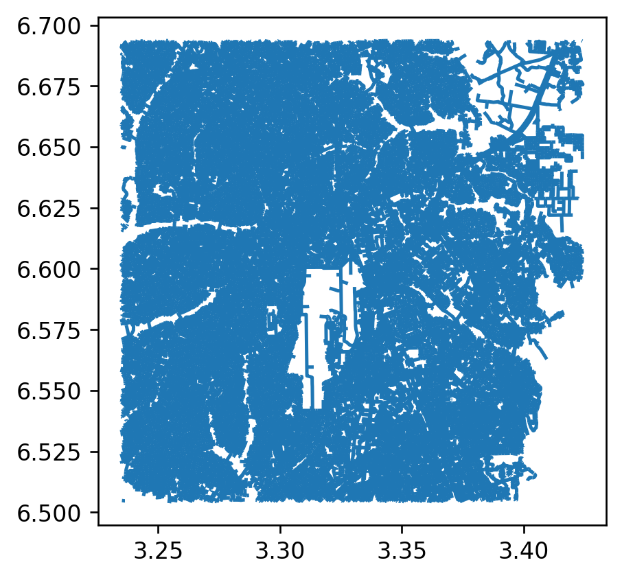

If you want to continue exploring the Roads dataset on the command line, proceed to the Roads network data processing notebook here: LINK.

You can also add the Feature Service directly in QGIS or ArcGIS Pro.

In QGIS, under Layer, choose Add Layer and then Add ArcGIS Feature Service Layer. Select new, give a name when prompted, and paste the Feature Server URL into the URL field. Select Connect, and then Add the layer to your map. You can save the layer locally by right clicking, selecting Export, and then Save Feature As. After selecting a format, you can you save the data to your computer.

In ArcGIS Pro, you can add the Feature Service by following a similar method. Under the Map tab, click Add Data and choose Data From Path. Paste the provided Feature Server URL and click Add to load the layer into your map.

This method provides you with the option to view the data from the GRID3 Data Hub on your map without saving the whole dataset locally automatically; you can query or filter before exporting in order to only download the portion of the Roads dataset that you are interested in.